Mixed-boundary linear elasticity

Static walkthrough · shared Python workflow

Gallery

This page presents one accepted bounded elasticity result. It does not solve in the browser. The visible deformation is caller-owned presentation, and the reference mesh remains visible as a text-labelled comparison.

Stage 1 🧱Problem and boundaries

Python authors the sole concrete $1\,\mathrm{m}\times1\,\mathrm{m}$ rectangle. The left edge has zero displacement; the right, lower, and upper edges have zero traction. A $16\times16$ caller-owned Cartesian mesh realizes the domain.

python

graph = eqiora.geometry.GeometryGraph()
rectangle = graph.rectangle(x_bounds=(0.0, 1.0), y_bounds=(0.0, 1.0))
geometry = graph.build(
    rectangle,
    named_topology={
        "body": rectangle.region,
        "x_lower": rectangle.boundaries[0],
        "x_upper": rectangle.boundaries[1],
        "y_lower": rectangle.boundaries[2],
        "y_upper": rectangle.boundaries[3],
    },
)

Shared installed-Python geometry and mesh workflow

Stage 2 🧩Eqiora model definition

The .eqi Component owns displacement, material parameters, load potential, equilibrium, and the four abstract supports. With displacement $\boldsymbol{u}$, shear modulus $\mu$, Lamé coefficient $\lambda$, and length $\ell$, its stress and load are

$$\boldsymbol{\sigma}(\boldsymbol{u}) =2\mu\,\operatorname{sym}(\nabla\boldsymbol{u}) +\lambda\,\operatorname{div}(\boldsymbol{u})\boldsymbol{I}, \qquad q=\frac{2\mu x}{\ell}.$$

The balance relation is

$$-\nabla\!\cdot\boldsymbol{\sigma}(\boldsymbol{u})-\nabla q=0.$$

Eqiora component source

Stage 3 🔷Typed numerical plan

The root resolver reads physics from the compiled Model. Python supplies Q1 spatial policy and one explicit linear-solve policy; neither selects a separate elasticity application type.

python

model = eqiora.compile(
    path=files(eqiora).joinpath("examples", "mixed-boundary-elasticity.eqi"),
    geometry=geometry,
    entry="MixedBoundaryElasticity2d",
    bindings={
        "body": geometry.selection("body"),
        **{
            side: (geometry.selection(side), geometry.selection("body"))
            for side in ("x_lower", "x_upper", "y_lower", "y_upper")
        },
        "mu": 3.0, "lambda": 0.0, "length_scale": 1.0,
    },
)
plan = eqiora.resolve(
    model,
    mesh=mesh,
    spatial=eqiora.fem.Q1(),
    solve=eqiora.solve.Linear(...),
)

Shared compile and resolve workflow

Stage 4 ▶Run and common Result

The shared function executes one direct root lifecycle and returns the exact Plan together with its common Result:

python

return plan, eqiora.run(plan)

The displacement is selected only by the Plan-owned field handle:

python

displacement = result.output(plan.capability.displacement)

The plotting path reuses that function; it does not restate geometry, physics, mesh generation, or solve policy.

Stage 5 📐Displacement presentation

Presentation, not evidence.Units: mDisplacement at scale 1, with the undeformed reference mesh shown for comparison.View the caller-owned plotting path

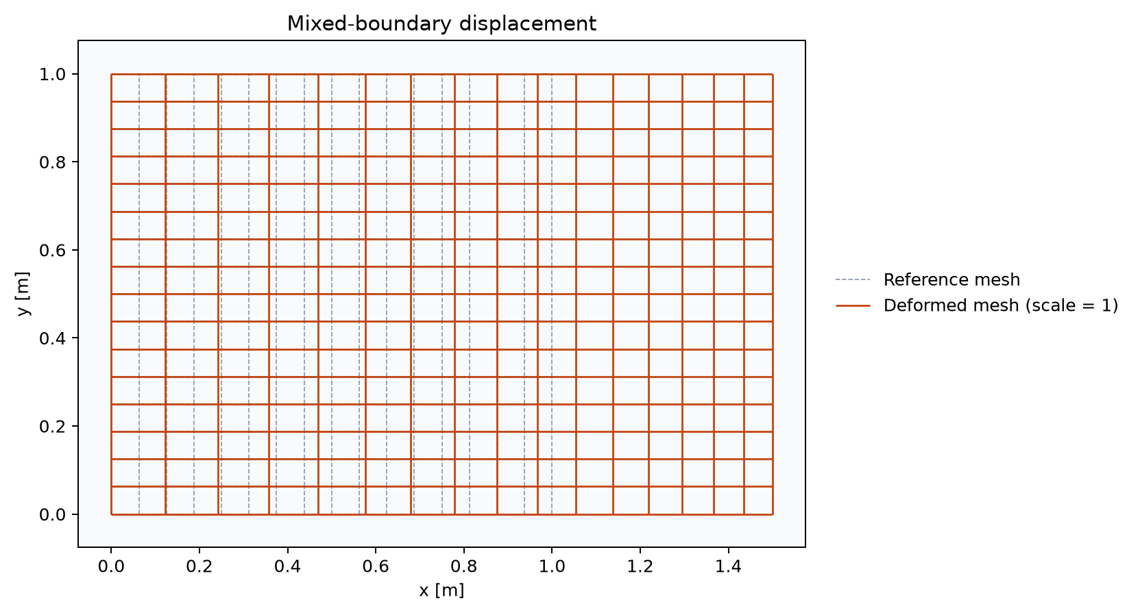
The dashed mesh is the reference geometry. The orange mesh adds the displacement with visible scale 1. The scale changes only presentation, never the Result. The static image contains no motion; the full alt text and this paragraph remain available when images are unavailable.

Stage 6 ✅Verification boundary

Verified boundary

Supported

• One bounded 2D mixed-boundary linear-elasticity workflow reaches a common Result and a caller-owned displacement figure through the root lifecycle.
• The installed product case checks the caller Geometry, common Plan/Result composition, Plan-owned displacement projection, and headless plot.
• The structural case independently owns the accepted scientific values and tolerances; publication does not derive them from pixels.

Not claimed

• This bounded 2D linear-elasticity workflow does not cover arbitrary boundary data, stress recovery, nonlinear or dynamic structure, or wider element families.
• It makes no convergence, performance, production-scale, or pixel-validation claim.

Installed-product dossier · Scientific evidence dossier · Read the human capability boundary · Find the checks behind this claim

Understand and reproduce the workflow

Read the lessons on constitutive laws and boundary and interface conditions, then follow the same structural model in the Python guide.