
Exact-cylinder steady Stokes
Build a two-dimensional steady Stokes model of flow past a cylinder, mesh it, and plot the pressure. The pressure field shows how pressure balances viscous stress around the obstacle.
Before you begin
Section titled “Before you begin”Follow Get started and keep its eqiora-source checkout and
.venv. From the folder containing both, add the mesh and plotting extras,
then run the example with the same Python environment:
uv add 'eqiora[gmsh,matplotlib]'uv run python eqiora-source/examples/python/exact_cylinder_stokes.py --pressure-png pressure.pngThe following stages explain the code and how to read the saved plot.
Stage 1 Problem setup
The fluid region is a channel with an exact authored circle centred at and radius . The problem is two-dimensional, steady, incompressible Stokes flow.
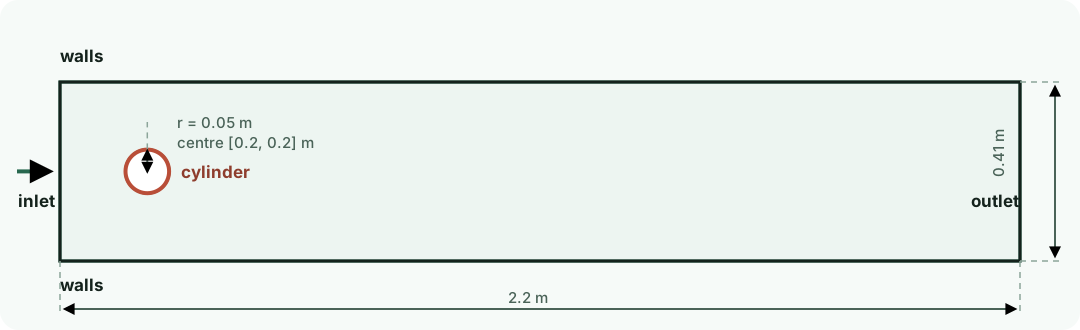
Exact authored geometry and boundary names. The later demonstration mesh approximates the circle with straight boundary segments.
The Python script builds that geometry explicitly:
geometry_graph = eqiora.geometry.GeometryGraph()rectangle = geometry_graph.rectangle(x_bounds=(0.0, 2.2), y_bounds=(0.0, 0.41))circle = geometry_graph.circle(center=(0.2, 0.2), radius=0.05)fluid = geometry_graph.subtract(rectangle, circle)geometry = geometry_graph.build( fluid, named_topology={ "fluid": fluid.region, "inlet": rectangle.boundaries[0], "outlet": rectangle.boundaries[1], "walls": rectangle.boundaries[2:], "cylinder": circle.boundaries[0], },)Stage 2 Eqiora model definition
Start with the Cauchy stress. With velocity , pressure , dynamic viscosity , identity tensor , and force potential :
Here ,
, and pressure has source unit
kg/(m*s^2), displayed as pascals. The Eqiora source below states the same model.
Eqiora source form
// Equations-only component for steady, incompressible flow around a cylinder.// The concrete channel and cylinder Geometry are authored separately in Python.public component SteadyFlowPastCylinder(  support fluid: volume(ambient_dimension = 2),  support inlet: boundary(parent = fluid),  support outlet: boundary(parent = fluid),  support walls: boundary(parent = fluid),  support cylinder: boundary(parent = fluid),  // Values supplied when the component is compiled into a Model.  parameter dynamic_viscosity: kg / (m * s),  parameter zero_pressure: kg / (m * s ^ 2),  parameter inlet_speed: m / s,  parameter channel_height: m) {  // Supports name the volume and its semantic boundaries without defining their shape.
  // Unknown continuum fields live on the fluid volume.
  variable velocity: vector<m / s, 2> on fluid in smooth;  variable pressure: kg / (m * s ^ 2) on fluid in h1;
  // Auxiliary fields keep prescribed forcing and profiles explicit and unit-checked.  variable force_potential: kg / (m * s ^ 2) on fluid;  variable inlet_profile: m / s on fluid in h1;
  relation force_definition on fluid {    force_potential - zero_pressure = 0;  }  relation inlet_profile_definition on fluid {    inlet_profile      - 4 * inlet_speed * coordinate(1) * (channel_height - coordinate(1))        / channel_height ^ 2 = 0;  }
  // Steady Stokes momentum balance and incompressibility in the fluid volume.  relation momentum on fluid {    -div(      2 * dynamic_viscosity * symmetric_part(grad(velocity))      - isotropic_lift(pressure)    ) - grad(force_potential) = 0;  }  relation incompressibility on fluid {    div(velocity) = 0;  }
  // Boundary laws: parabolic inlet, traction-free outlet, and no-slip walls.  relation inlet_velocity on inlet {    trace(velocity) + normal(isotropic_lift(inlet_profile)) = 0;  }  relation outlet_traction on outlet {    normal(      2 * dynamic_viscosity * symmetric_part(grad(velocity))      - isotropic_lift(pressure)    ) = 0;  }  relation wall_velocity on walls { trace(velocity) = 0; }  relation cylinder_velocity on cylinder { trace(velocity) = 0; }}
Complete cylinder model · Reusable incompressible balance component
Compile the component with the geometry used for meshing:
model = eqiora.compile( path=files(eqiora).joinpath("examples", "steady-flow-past-cylinder.eqi"), geometry=geometry, entry="SteadyFlowPastCylinder", bindings={ "fluid": geometry.selection("fluid"), **{ side: (geometry.selection(side), geometry.selection("fluid")) for side in ("inlet", "outlet", "walls", "cylinder") }, "dynamic_viscosity": 1.0e-3, "zero_pressure": 0.0, "inlet_speed": 0.3, "channel_height": 0.41, },)Stage 3 Mesh and boundaries
The inlet profile uses and channel height :
At the outlet, . The walls and cylinder use .
The full source above attaches these relations to fluid, inlet, outlet,
walls, and cylinder. At the left inlet, the outward normal points left,
so trace(velocity) + normal(isotropic_lift(inlet_profile)) = 0 directs flow
into the channel. The outlet law balances pressure and viscous traction together;
it does not separately prescribe zero pressure and zero velocity gradient.
Request at most 50 circular-boundary facets, then generate the mesh:
mesh_request = eqiora.meshing.GmshMesher( maximum_boundary_error=1e-4, maximum_target_size=0.025, minimum_mean_ratio=1e-5, maximum_boundary_facets=50,)mesh_plan = eqiora.meshing.resolve(geometry, mesh_request)mesh = eqiora.meshing.generate(mesh_plan)Stage 4 Submit and result
Combine the Model and Mesh with the MINI/P1 element and linear-solve
settings; with scaling=None, Eqiora derives the scaling. Running the resulting
Plan returns a Result.
linear = eqiora.solve.Linear( algorithm=eqiora.solve.LinearSolver.SparseLu, preconditioner=eqiora.solve.Preconditioner.Identity, reduction=eqiora.solve.Reduction.Fast, provider=eqiora.solve.SolverProvider.faer(), relative_tolerance=1e-6, absolute_tolerance=1e-13, maximum_iterations=10_000,)plan = eqiora.resolve( model, mesh=mesh, spatial=eqiora.fem.MiniP1(), solve=linear, scaling=None,)result = eqiora.run(plan)Stage 5 Pressure visualization
The plotting cell selects the pressure FieldOutput from the
Result and passes it to the general scalar-field adapter:
pressure = result.output(plan.capability.pressure)pressure_figure = eqplot.plot_scalar_field(result, field=plan.capability.pressure)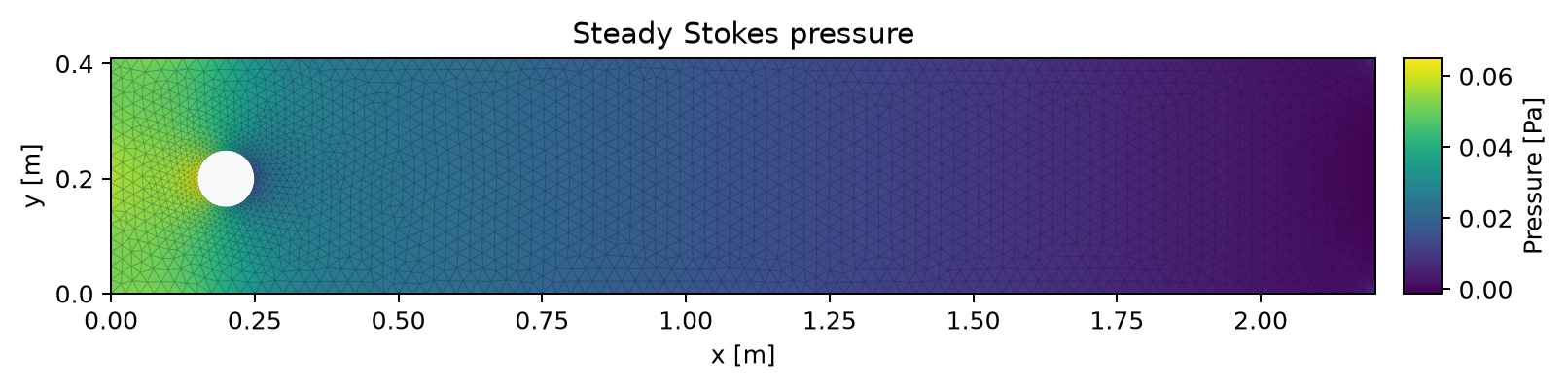
Stage 6 Reading the pressure plot
Pressure is shown in pascals. Use the color scale to compare the pressure upstream and downstream of the cylinder. This steady Stokes model omits inertial effects, so use the transient example to explore evolving flow.
Next steps
Section titled “Next steps”Derive the model in Stokes flow and boundaries and study pressure coupling and refinement. The modeling guide runs the same cylinder problem step by step in Python, and the language reference defines the equation syntax.