5. Computing incompressible flow

The question

The model now has equations, a domain and boundary laws. How do we obtain numbers, and which observations tell us whether changing the numerical method matters? Keep the physical problem fixed while choosing its numerical realization.

From strong balance to a mixed problem

Multiply steady momentum by a test velocity $\boldsymbol v$ that vanishes on prescribed-velocity boundaries. Integration by parts gives

$$\int_\Omega 2\mu\boldsymbol D(\boldsymbol u):\boldsymbol D(\boldsymbol v)\,\mathrm dV -\int_\Omega p\,\nabla\cdot\boldsymbol v\,\mathrm dV =\int_\Omega\boldsymbol f\cdot\boldsymbol v\,\mathrm dV +\int_{\Gamma_t}\boldsymbol t\cdot\boldsymbol v\,\mathrm dA.$$

The continuity equation is tested with a scalar $q$: $\int_\Omega q\nabla\cdot\boldsymbol u\,\mathrm dV=0$. Velocity and pressure therefore form a coupled, or mixed, system. Pressure acts as the field enforcing the divergence constraint.

A finite-element method approximates these fields in finite-dimensional spaces. The example uses MINI/P1: continuous piecewise-linear velocity enriched with a cell bubble, paired with continuous piecewise-linear pressure. The bubble vanishes on the triangle’s edges and enriches its interior velocity. The pairing addresses the stability of the velocity–pressure coupling; choosing unrelated spaces merely because they interpolate smoothly can produce spurious pressure patterns. See the original MINI-element paper.

A finite-volume formulation instead foregrounds balances over cells and shared face fluxes. Both methods approximate the continuum model; their conservation, accuracy and computational costs must be examined for the actual realization. The current cylinder run uses the stated finite-element method.

Run the investigation

Complete Get started first, retaining its eqiora-source checkout and .venv. Work from the same folder. Add the geometry and plotting extras to that exact source installation:

bash

uv pip install --python .venv/bin/python --reinstall-package eqiora './eqiora-source[gmsh,matplotlib]'
uv run --no-project --python .venv/bin/python python eqiora-source/examples/python/exact_cylinder_stokes.py --pressure-png pressure.png

The script compiles the equations, generates a triangular mesh, resolves the MINI/P1 plan, runs the linear solve and writes pressure.png. Its full explanation lives in the steady-cylinder walkthrough.

Read the Python workflow. Change parameters or numerical settings there, keeping the installed source revision and the script together.

Pressure from the steady workflow. Compare the upstream and downstream regions using the same colour scale.

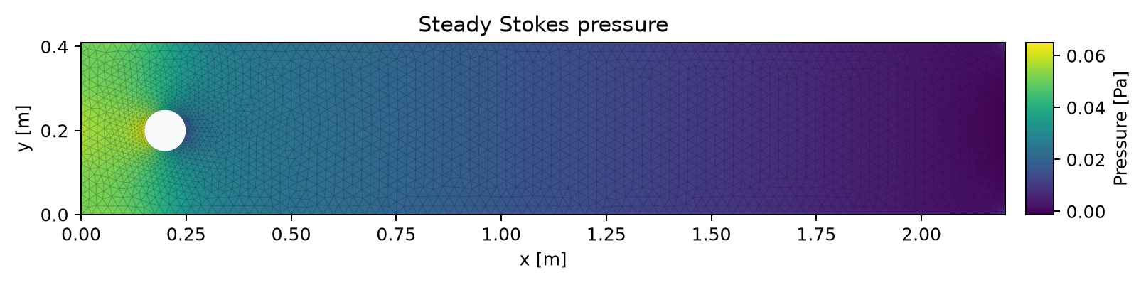
Before interpreting pressure magnitudes, recover the model’s viscosity, inlet speed and outlet traction. A plot without those quantities is missing part of the problem definition.

Read the source as a chain of decisions

Object	Decision it records
Model	Unknowns, units, equations and boundary relations
Geometry	Exact domain and named selections
Mesh	Discrete geometric representation
Plan	Model plus spatial method, solver settings and scaling
Result	Fields and observations produced by the run

This separation lets you refine the mesh without rewriting Newtonian stress. It also makes it possible to change a physical law deliberately without pretending that the resulting difference is numerical error.

Choose an observation before refinement

For this problem, inlet flux is known independently from the prescribed parabola. Compare integrated outlet flux with that value. Pressure drop and surface force ask different questions: pressure differences use values at specified positions, while traction involves pressure and velocity derivatives. Agreement of one observation does not establish accuracy of all the others.

Three distinct approximations need attention:

• Geometry and spatial approximation: triangles and straight boundary segments approximate the domain and fields. Changing a target mesh size alone may leave the circular boundary approximation nearly unchanged.
• Algebraic solve: a linear or nonlinear solve stops at a finite residual. Tightening that tolerance does not refine the physical discretization.
• Time approximation: transient methods add an error absent from this steady run. Reducing it requires changing the time step, not the video frame rate.

For a quantity $J$, compare $J_h$, $J_{h/2}$ and $J_{h/4}$ while maintaining a consistent geometric refinement family. If $J_h=J_*+Ch^p$ in the asymptotic regime, then

$$\frac{|J_h-J_{h/2}|}{|J_{h/2}-J_{h/4}|}\approx2^p.$$

This is a hypothesis to test, not a reason to assign a convergence order from just two runs. A target size is not necessarily the largest realized edge, so record the generated mesh as well as its requested settings. The numerical-simulation book develops error comparisons in problems with simpler reference solutions.

A small investigation

Use the steady script for a linearity experiment before attempting a large refinement campaign. Predict the consequence of changing the maximum inlet speed from $0.3$ to $0.15\,\mathrm{m/s}$, with viscosity and geometry fixed. Reuse the same mesh settings and compare pressure with the same colour scale: the Stokes equations predict half the velocity and half the pressure relative to the unchanged zero-traction reference.

Then restore the speed and double viscosity. Velocity should be unchanged and pressure should double. These predictions follow from the linear boundary problem, not from the first computed image.

Exercises

1. Why might pressure look smooth even when wall traction is poorly resolved?
2. A smaller linear residual leaves a pressure-drop observation unchanged. Which uncertainty has been reduced, and which has not?
3. Explain why doubling the number of mesh cells does not necessarily halve a two-dimensional characteristic edge length.
4. Design a table for a future refinement study. Include the actual mesh, observation definition, requested tolerance and observed quantity.

Check your reasoning. Derivatives amplify unresolved field variation, so traction can be more sensitive than pressure values. In a uniform two-dimensional refinement, halving lengths multiplies the cell count approximately by four.

Previous: Stokes flow and boundaries · Book map · Next: Cylinder wakes