6. Cylinder wakes

The question

Fluid leaving a cylinder carries momentum and vorticity downstream. To describe that process, restore temporal storage and advective momentum transport to the steady model. First inspect the destination; then derive what changed.

One state from the transient investigation. The lower panel connects the spatial pattern to cylinder lift over physical time.

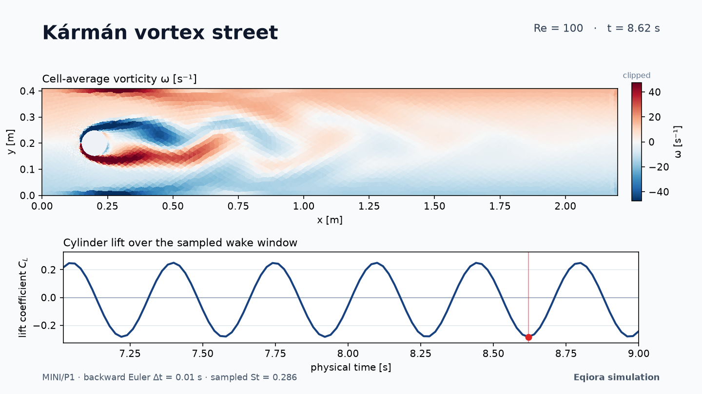
The Gallery video follows the same type of observation through successive states. Read the colour scale: vorticity is a signed quantity with units of inverse seconds, not speed.

Restore the missing momentum terms

For constant density,

$$\rho\partial_t\boldsymbol u+ \nabla\cdot(\rho\boldsymbol u\otimes\boldsymbol u) -\nabla\cdot\boldsymbol\sigma-\boldsymbol f=0, \qquad \nabla\cdot\boldsymbol u=0.$$

Incompressibility makes the advective divergence equal to $\rho(\boldsymbol u\cdot\nabla)\boldsymbol u$ in the smooth continuum equations. The product of velocity with itself makes this term nonlinear. Retaining $\partial_t\boldsymbol u$ but omitting this transport term gives unsteady Stokes flow; the presence of a time integrator alone does not make it Navier–Stokes flow.

In two dimensions, define scalar vorticity $\omega=\partial_xu_y-\partial_yu_x$. Taking the curl of momentum for constant properties and a conservative body force yields

$$\partial_t\omega+\boldsymbol u\cdot\nabla\omega=\nu\nabla^2\omega.$$

Pressure drops out of this interior equation because the curl of a gradient is zero. Pressure remains essential to incompressibility and boundary forces. Viscous wall motion and no-slip conditions are also essential to how vorticity enters the flow; this equation alone is not a complete boundary specification.

Calculate the scales before running

The example uses $D=0.1\,\mathrm m$, mean inlet speed $\bar U=1\,\mathrm{m/s}$, $\rho=1\,\mathrm{kg/m^3}$ and $\mu=0.001\,\mathrm{Pa\,s}$. The maximum of its parabolic inlet is $1.5\,\mathrm{m/s}$. Therefore

$$\mathrm{Re}=\frac{\rho\bar UD}{\mu}=100,\quad T_c=\frac D{\bar U}=0.1\,\mathrm s,\quad T_\nu=\frac{D^2}{\nu}=10\,\mathrm s.$$

Their ratio $T_\nu/T_c=\mathrm{Re}$ compares viscous diffusion over one diameter with convection over that diameter. The $2.2\,\mathrm m$ channel has a different advection scale, approximately $2.2\,\mathrm s$ at the mean inlet speed. A run lasting one diameter transit is short compared with a channel transit.

The cylinder centre is at $y=0.2\,\mathrm m$, slightly below the channel centre $0.205\,\mathrm m$. Exact reflection symmetry is therefore absent in this geometry. In a different, perfectly symmetric setup, an exactly symmetric initial state can conceal an unstable antisymmetric mode until a perturbation is introduced or grows. Record such changes as changes to the experiment.

Read the direct source, then identify the reusable pieces

transient-flow-past-cylinder.eqi

public operator outer_product(input left: spatial[1], input right: spatial[1]): spatial[2]
  = component(left, 0) * component(right, 1);

public component TransientFlowPastCylinder(
  support fluid: volume(ambient_dimension = 2),
  support inlet: boundary(parent = fluid),
  support outlet: boundary(parent = fluid),
  support walls: boundary(parent = fluid),
  support cylinder: boundary(parent = fluid),
  parameter density: kg / m ^ 3,
  parameter dynamic_viscosity: kg / (m * s),
  parameter zero_pressure: kg / (m * s ^ 2),
  parameter inlet_speed: m / s,
  parameter channel_height: m
) {
  state velocity: vector<m / s, 2> on fluid;
  variable pressure: kg / (m * s ^ 2) on fluid;
  variable force_potential: kg / (m * s ^ 2) on fluid;
  variable inlet_profile: m / s on fluid;

  relation force_definition on fluid {
    force_potential - zero_pressure = 0;
  }
  relation inlet_profile_definition on fluid {
    inlet_profile
      - 4 * inlet_speed * coordinate(1) * (channel_height - coordinate(1))
        / channel_height ^ 2 = 0;
  }
  relation momentum on fluid {
    density * derivative(velocity)
      + div(density * outer_product(left = velocity, right = velocity))
      - div(
        2 * dynamic_viscosity * symmetric_part(grad(velocity))
        - isotropic_lift(pressure)
      ) - grad(force_potential) = 0;
  }
  relation incompressibility on fluid {
    div(velocity) = 0;
  }

  relation inlet_velocity on inlet {
    trace(velocity) + normal(isotropic_lift(inlet_profile)) = 0;
  }
  relation outlet_traction on outlet {
    normal(
      2 * dynamic_viscosity * symmetric_part(grad(velocity))
      - isotropic_lift(pressure)
    ) = 0;
  }
  relation wall_velocity on walls { trace(velocity) = 0; }
  relation cylinder_velocity on cylinder { trace(velocity) = 0; }
}

Compared with the steady source, velocity is now a state, density is an explicit parameter, and the momentum relation contains both its derivative and advective flux. The same Newtonian stress and boundary relations remain visible. The local outer_product declaration supplies the tensor product used by that flux.

Open the transient model. After understanding the direct equations, compare the standard inertial-flow component: it packages temporal inertia and viscous balance but omits advective transport. Its shorter name cannot substitute for inspecting which terms it supplies.

Run and interpret physical time

Use the same source installation and extras as Chapter 5. From the folder containing .venv and eqiora-source, run:

bash

uv run --no-project --python .venv/bin/python python eqiora-source/examples/python/karman_vortex_street.py --vorticity-png wake.png

The complete workflow begins from a steady Stokes field, advances 700 steps of $0.01\,\mathrm s$, then samples another 200 steps. It saves observations every two steps during the final interval. Thus the final time is $9\,\mathrm s$ and sample spacing is $0.02\,\mathrm s$. The warm-up time is part of the physical trajectory, even though most of those states are not retained for plotting.

Read initialization, time stepping and observation code. A short run can exercise the workflow but cannot answer a question about a long-time oscillation. Likewise, increasing video frames per second changes playback; it does not reduce the integration step or lengthen physical time.

Measure force and frequency

The force of fluid on the cylinder is opposite to the force of the cylinder on the fluid. With the fluid region’s outward normal at the hole, $\boldsymbol F'=-\int_{\Gamma_c}\boldsymbol\sigma\boldsymbol n\,\mathrm ds$. The prime emphasizes force per unit span in $\mathrm{N/m}$. The workflow selects the force on the cylinder and computes

$$C_D=\frac{2F'_x}{\rho\bar U^2D},\qquad C_L=\frac{2F'_y}{\rho\bar U^2D},\qquad \mathrm{St}=\frac{fD}{\bar U}=\frac{D}{\bar UT}.$$

$T$ is an oscillation period in seconds. The script estimates it from repeated rising crossings of the mean-centred lift signal. Too few crossings leave the estimate undefined; a numerical value from a short window may still depend on startup, window placement and sampling. Examine the trace before interpreting its frequency.

A uniform pressure offset cancels from the force integrated around a closed cylinder because $\int_{\Gamma_c}\boldsymbol n\,\mathrm ds=0$. It also cancels from front-minus-rear pressure. This does not permit changing pressure alone while retaining an incompatible outlet traction.

Compare like physical problems

The DFG 2D-2 specification provides the channel geometry and Reynolds-100 comparison problem. Before comparing numbers, inspect its outlet law, initialization and measurement window. Its do-nothing outlet uses $\nu\nabla\boldsymbol u-p\boldsymbol I$, whereas this model prescribes the full symmetric Newtonian traction. Those boundary expressions must not be identified merely because the interior incompressible equations can both be written using a velocity Laplacian.

The present method is MINI/P1 with Backward Euler. Backward Euler adds temporal damping; the selected spatial method and geometric approximation also affect forces and oscillations. A useful next experiment separates these effects: reduce the time step at fixed mesh and physical window, then compare meshes at a suitably small time step. Finally shift or extend the observation window to examine whether the measured oscillation has settled. Visual similarity of two wakes does not answer those quantitative questions.

Exercises

1. Recompute Reynolds number incorrectly using the maximum inlet speed. What value results, and which convention caused the discrepancy?
2. A lift trace has a period of $0.4\,\mathrm s$ at the stated $D$ and $\bar U$. Compute its Strouhal number. Treat this as a hypothetical signal.
3. Halve the time step while preserving physical warm-up and sampling durations. How must the step counts change? What about the output stride if you want the same physical sample spacing?
4. A refined mesh gives a smoother wake but unchanged observation duration. Which possible errors remain unresolved?

Check your reasoning. Exercise 1 gives 150 instead of the mean-speed value 100. Exercise 2 gives $\mathrm{St}=0.25$. In exercise 3, double both step counts and the output stride. More cells alone do not resolve time discretization or an unsettled observation window.

Previous: Computing incompressible flow · Book map · References and further study