Kármán vortex street

Gallery

Follow a two-dimensional incompressible Navier–Stokes simulation as vortices form behind a circular cylinder and travel downstream. The image and video show Eqiora output from the linked workflow.

Before you begin

Follow Get started and keep its eqiora-source checkout and .venv. From the folder containing both, install the mesh and plotting extras and save the final vorticity field:

bash

uv pip install --python .venv/bin/python --reinstall-package eqiora './eqiora-source[gmsh,matplotlib]'
uv run --no-project --python .venv/bin/python python eqiora-source/examples/python/karman_vortex_street.py --vorticity-png wake.png

The Python source includes geometry, model compilation, initialization, time integration and observations. The stages below explain that same workflow.

Stage 1 🧭Define the channel and cylinder

Python authors the exact $2.2\,\mathrm{m}\times0.41\,\mathrm{m}$ channel and subtracts a circle of diameter $0.1\,\mathrm{m}$ centered at $(0.2\,\mathrm{m}, 0.2\,\mathrm{m})$. The Geometry names the fluid, inlet, outlet, walls, and cylinder selections used throughout the run.

python

graph = eqiora.geometry.GeometryGraph()
rectangle = graph.rectangle(x_bounds=(0.0, 2.2), y_bounds=(0.0, 0.41))
circle = graph.circle(center=(0.2, 0.2), radius=0.05)
fluid = graph.subtract(rectangle, circle)
geometry = graph.build(fluid, named_topology={...})

View the complete plain-Python workflow

Stage 2 🧩Set the flow problem

The .eqi source defines transient incompressible Navier–Stokes equations, no-slip walls and cylinder, a parabolic inlet, and a zero-traction outlet. The physical setup uses density 1 kg/m³, dynamic viscosity 0.001 Pa·s, and maximum inlet speed 1.5 m/s. With mean inlet speed 1 m/s and cylinder diameter 0.1 m, the Reynolds number is $\mathrm{Re}=\rho\bar U D/\mu=100$.

The outlet condition is authored in the same .eqi source: $(2\mu\,\mathrm{sym}(\nabla u)-pI)n=0$, where $n$ is the outward normal.

Open the Eqiora source

Stage 3 🔷Generate the mesh

The workflow asks Gmsh for an unstructured triangular mesh while retaining the exact named geometry needed for boundary conditions and observations. Its characteristic-size target is $h=0.02\,\mathrm{m}$.

python

request = eqiora.meshing.GmshMesher(
    maximum_boundary_error=1e-4,
    maximum_target_size=0.02,
    minimum_mean_ratio=1e-5,
    maximum_boundary_facets=50,
)
mesh = eqiora.meshing.generate(eqiora.meshing.resolve(geometry, request))

Compare meshes using a fixed physical observation window, then vary the time step separately. Pressure, force and frequency can respond differently to these changes; a smoother image alone does not measure their accuracy.

Stage 4 ▶Advance the wake

Numerical method

The resolved plan combines MINI/P1 elements, Backward Euler time stepping, Newton iteration, a sparse linear solver, and incompressible-flow scaling. Starting from a steady Stokes field, it advances 700 steps of 0.01 s, then samples another 200 steps through 9 s. Saving every second step gives a 0.02 s interval between displayed states. Video playback speed changes how quickly you watch them, not their physical times.

python

plan = eqiora.resolve(
    model,
    mesh=mesh,
    spatial=eqiora.fem.MiniP1(),
    temporal=eqiora.time.BackwardEuler(0.01),
    solve=eqiora.solve.Newton(linear=linear),
    scaling=eqiora.fluid.IncompressibleScaling(...),
)
result = eqiora.run(plan, state=state, steps=steps, output_steps=output_steps)

The geometry and Reynolds number follow the FeatFlow DFG 2D-2 specification. For numerical comparisons, also inspect the boundary laws and measurement window: this model uses full symmetric Newtonian outlet traction and begins from a Stokes field. The reference uses a different outlet expression and initialization procedure, as well as different spatial and temporal methods. The cylinder-wake lesson explains how these choices affect a comparison.

Stage 5 📐Inspect vorticity and loads

Cell-average curl exposes the rotating structures convected behind the cylinder. The same states provide signed cylinder force and pressure samples at the front and rear of the obstacle.

python

accepted = result.trajectory.states[-1]
vorticity = accepted.curl(plan.capability.velocity)
cylinder_force = accepted.boundary_force(geometry.selection("cylinder"))
front_pressure = accepted.sample(plan.capability.pressure, at=(0.15, 0.2))
rear_pressure = accepted.sample(plan.capability.pressure, at=(0.25, 0.2))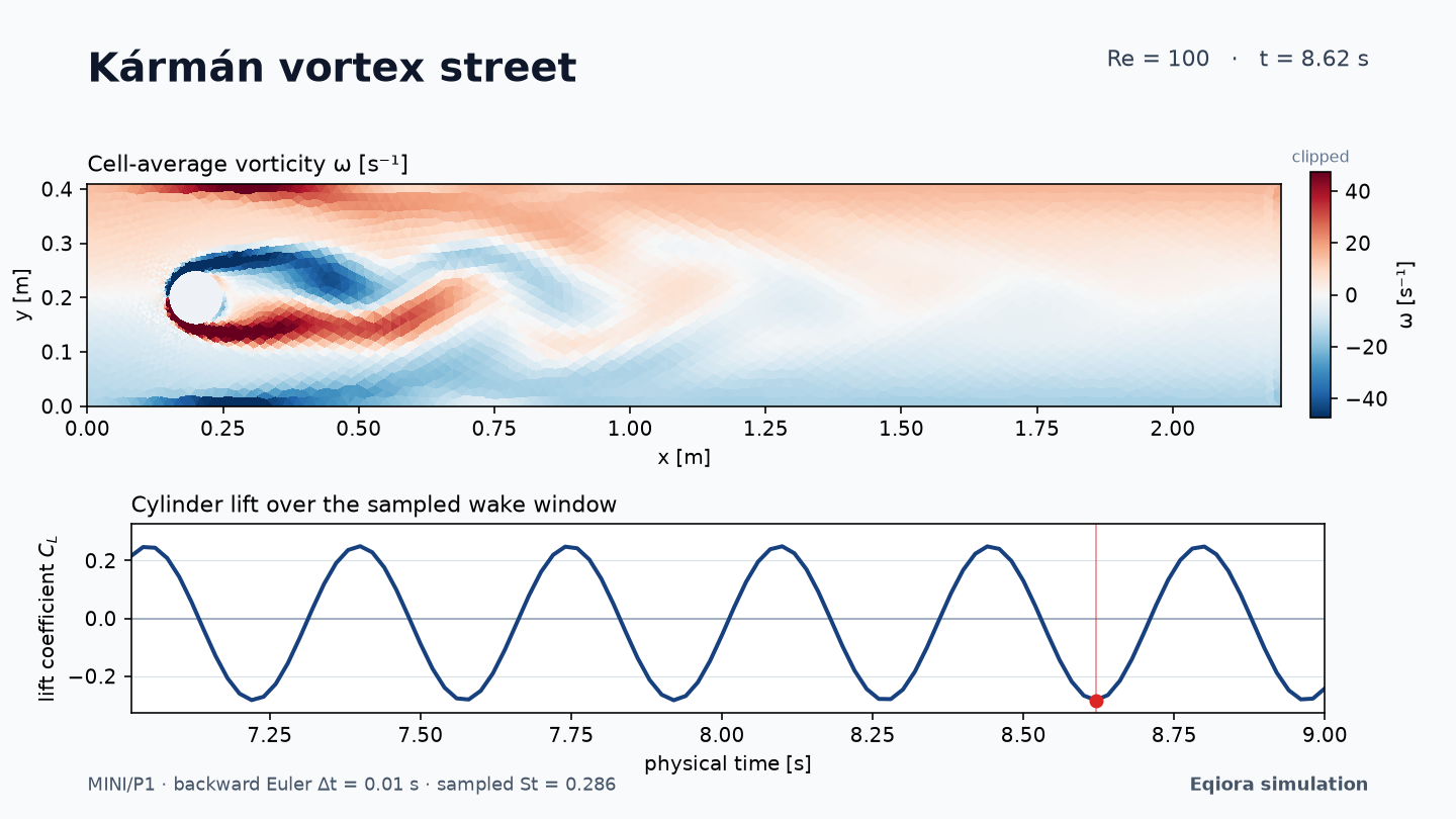

Units: s⁻¹A transient state, colored by cell-average vorticity.View the media producer

Stage 6 🎞️Follow the vortex street

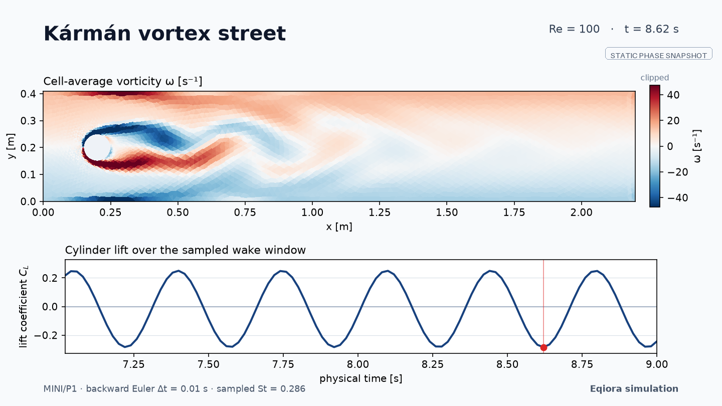
Cell-average vorticity from selected states. Motion is disabled when the browser requests reduced motion; one representative state is shown instead.

Oppositely rotating structures form behind the obstacle. Their alternating signed vorticity travels downstream through the channel as the transient run advances.

Understand and reproduce the workflow

Derive the momentum terms and interpret force histories in Cylinder wakes. The Python execution guide explains run control, diagnostics and arrays. Use the linked Python source with the installation above to reproduce the workflow.