4. Stokes flow and boundaries

The question

Place a cylinder inside the channel. The flow must turn around it, so the parallel-flow calculation no longer applies. Which terms should we retain, and what does the outlet mean physically?

Compare inertia with viscosity

Choose a speed $U$ and length $L$. Advective inertia scales as $\rho U^2/L$, while viscous force per volume scales as $\mu U/L^2$. Their ratio is

$$\mathrm{Re}=\frac{\rho UL}{\mu}=\frac{UL}{\nu}.$$

At small Reynolds number, for a steady flow, neglecting inertia leaves

$$-\nabla\cdot\boldsymbol\sigma=\boldsymbol f, \qquad \nabla\cdot\boldsymbol u=0, \qquad \boldsymbol\sigma=2\mu\operatorname{sym}(\nabla\boldsymbol u)-p\boldsymbol I.$$

These are the steady Stokes equations. Small Reynolds number alone does not justify neglecting rapid temporal changes: on an imposed time scale $T$, the unsteady-to-viscous ratio is $L^2/(\nu T)$. A rapidly oscillating low-speed flow may need unsteady Stokes equations.

For a homogeneous Stokes boundary problem driven only by an imposed inlet velocity, doubling that velocity doubles velocity and pressure; changing viscosity scales pressure while leaving the velocity solution unchanged. The traction data must scale consistently. This linearity provides a useful prediction even when the full spatial field has no simple formula.

Define the geometry and boundaries

The geometry supplies named regions to which the mathematical boundary laws attach.

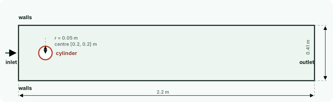
The steady example chooses the inlet profile

$$\boldsymbol u_{\rm in}(y)=\left(\frac{4U_{\max}y(H-y)}{H^2},0\right), \qquad U_{\max}=0.3\,\mathrm{m/s},\quad H=0.41\,\mathrm m.$$

From Chapter 3, the mean inlet speed is $0.2\,\mathrm{m/s}$ and the volume flux per unit span is $0.082\,\mathrm{m^2/s}$. Steady incompressibility requires the same integrated outlet flux. These values are available before any solve.

At the cylinder and walls, no slip sets $\boldsymbol u=0$. At the outlet, $\boldsymbol\sigma\boldsymbol n=0$ prescribes a traction. It does not separately impose both $p=0$ and zero velocity gradient. The pressure and viscous contributions combine to satisfy the one vector condition.

The Stokes model contains no density parameter. It deliberately omits inertia; entering a large inlet speed does not add that missing term. Use a density and physical scales to assess applicability before treating a Stokes result as a prediction for an actual fluid.

Write the mathematics in Eqiora

The complete source expresses precisely those fields and laws:

steady-flow-past-cylinder.eqi

// Equations-only component for steady, incompressible flow around a cylinder.
// The concrete channel and cylinder Geometry are authored separately in Python.
public component SteadyFlowPastCylinder(
  support fluid: volume(ambient_dimension = 2),
  support inlet: boundary(parent = fluid),
  support outlet: boundary(parent = fluid),
  support walls: boundary(parent = fluid),
  support cylinder: boundary(parent = fluid),
  // Values supplied when the component is compiled into a Model.
  parameter dynamic_viscosity: kg / (m * s),
  parameter zero_pressure: kg / (m * s ^ 2),
  parameter inlet_speed: m / s,
  parameter channel_height: m
) {
  // Supports name the volume and its semantic boundaries without defining their shape.

  // Unknown continuum fields live on the fluid volume.

  variable velocity: vector<m / s, 2> on fluid;
  variable pressure: kg / (m * s ^ 2) on fluid;

  // Auxiliary fields keep prescribed forcing and profiles explicit and unit-checked.
  variable force_potential: kg / (m * s ^ 2) on fluid;
  variable inlet_profile: m / s on fluid;

  relation force_definition on fluid {
    force_potential - zero_pressure = 0;
  }
  relation inlet_profile_definition on fluid {
    inlet_profile
      - 4 * inlet_speed * coordinate(1) * (channel_height - coordinate(1))
        / channel_height ^ 2 = 0;
  }

  // Steady Stokes momentum balance and incompressibility in the fluid volume.
  relation momentum on fluid {
    -div(
      2 * dynamic_viscosity * symmetric_part(grad(velocity))
      - isotropic_lift(pressure)
    ) - grad(force_potential) = 0;
  }
  relation incompressibility on fluid {
    div(velocity) = 0;
  }

  // Boundary laws: parabolic inlet, traction-free outlet, and no-slip walls.
  relation inlet_velocity on inlet {
    trace(velocity) + normal(isotropic_lift(inlet_profile)) = 0;
  }
  relation outlet_traction on outlet {
    normal(
      2 * dynamic_viscosity * symmetric_part(grad(velocity))
      - isotropic_lift(pressure)
    ) = 0;
  }
  relation wall_velocity on walls { trace(velocity) = 0; }
  relation cylinder_velocity on cylinder { trace(velocity) = 0; }
}

Read it from the inside out:

1. velocity and pressure are unknown fields on the fluid region. Their dimensions are part of their declarations.
2. symmetric_part(grad(velocity)) is $\boldsymbol D$; isotropic_lift(pressure) is $p\boldsymbol I$.
3. force_potential has pressure units. Its gradient supplies a volume force. Here it is constant, so that force is zero. It is not the pressure unknown.
4. trace restricts a field to a boundary and normal contracts with the parent region’s outward normal.
5. At the left inlet $\boldsymbol n=(-1,0)$, so trace(velocity) + normal(isotropic_lift(inlet_profile)) = 0 prescribes a positive streamwise velocity. The plus sign is intentional.

Open the complete source. The source names supports but does not define a circle or a mesh. The Python workflow supplies the geometry and binds each support to its named selection.

Recognize the reusable law

Now that you have assembled the equations, open the incompressible standard source. Its SteadyStokesWithPotential2d component packages the same momentum and incompressibility relations. A containing model binds its support, fields and viscosity to those arguments; geometry and boundary conditions still belong to the containing problem.

The general fluid source also separates the balance from velocity/traction interfaces and wall laws. This is what reuse buys: you can read a named law as an abbreviation for equations you already understand. Use the standard-package reference for the runnable bundled Eqiora.Fluid.Incompressible composition. The cylinder example keeps the direct equations visible, so it remains a convenient place to study each term.

Pressure gauge: a boundary-dependent question

With prescribed velocity everywhere, adding a constant to pressure changes no interior pressure gradient. A pressure reference is then needed. A prescribed traction changes by $-C\boldsymbol n$ under $p\mapsto p+C$; it can fix that freedom. Do not introduce an extra arbitrary pressure condition without first checking what the existing boundary laws already determine.

Exercises

1. Integrate the inlet parabola and recover $0.082\,\mathrm{m^2/s}$.
2. At a right-hand boundary, what velocity direction would the same normal-inlet relation prescribe? Explain using its outward normal.
3. Which part of the source changes when a wall moves? Which part changes when viscosity depends on shear rate?
4. Why can the steady source not produce a time-evolving vortex street, however fine its mesh becomes?

Check your reasoning. A right-hand normal inlet points left into the region. Moving a wall changes a boundary law; non-Newtonian viscosity changes the constitutive law. Mesh refinement cannot introduce terms absent from the model.

Previous: Exact parallel flows · Book map · Next: Computing incompressible flow