4. A square with mixed boundaries

Where should the square move most?

Hold the left edge of a square and apply a uniform rightward body force. Keep the other three edges free of traction. The right edge should move most, but the material near the support should carry the greatest tensile stress: it must transmit the load from all the material to its right.

We will calculate both statements before running a solve. The two-dimensional model has displacement $\boldsymbol u$ in m, strain $\boldsymbol\varepsilon=\operatorname{sym}(\nabla\boldsymbol u)$ , and stress $\boldsymbol\sigma=2\mu\boldsymbol\varepsilon+ \lambda(\nabla\cdot\boldsymbol u)\boldsymbol I$ in Pa. Traction is $\boldsymbol\sigma\boldsymbol n$ , with outward normal $\boldsymbol n$ . See strain and stress for a local derivation of those definitions.

Conceptual boundary and load diagram. Here L = H = ℓ = 1 m. Arrows show force direction; their length is not a displacement or a computed value.

Build the equations

Use $0\le x\le L$ , $0\le y\le H$ , with $L=H=1\,\mathrm{m}$ . Set $\mu=3\,\mathrm{Pa}$ and $\lambda=0\,\mathrm{Pa}$ . Define the scalar load potential

q(x)=\frac{2\mu x}{\ell},\qquad \ell=1\,\mathrm{m}.

$q$ has units of Pa. Its gradient is the body force $\boldsymbol b=(2\mu/\ell,0)=(6,0)\,\mathrm{N/m^3}$ . The field $q$ is a convenient way to state this conservative load; it is not an unknown pressure exerted on the outer edges. The balance is

-\nabla\cdot\boldsymbol\sigma-\nabla q=\boldsymbol0.

At $x=0$ prescribe $\boldsymbol u=\boldsymbol0$ . On $x=L$ , $y=0$ and $y=H$ , prescribe $\boldsymbol\sigma\boldsymbol n=\boldsymbol0$ . No traction is prescribed at the fixed edge: its reaction is part of the answer.

Derive the answer on paper

Try $\boldsymbol u=(f(x),0)$ . With $\lambda=0$ , only $\sigma_{xx}=2\mu f'(x)$ is nonzero, so the horizontal free boundaries are automatically satisfied. The remaining equation and conditions reduce to

-2\mu f''(x)=\frac{2\mu}{\ell},\qquad f(0)=0,\qquad f'(L)=0.

Integrate once: $f'(x)=(L-x)/\ell$ . Integrate again:

\boxed{u_x(x,y)=\frac{Lx-x^2/2}{\ell},\quad u_y(x,y)=0},\qquad \sigma_{xx}=\frac{2\mu}{\ell}(L-x).

At $x=L/2$ , displacement is $0.375\,\mathrm{m}$ ; at $x=L$ , it is $0.5\,\mathrm{m}$ . These deliberately simple coefficients make a large deformation in a linear model. The result is a useful analytic test problem; it is not a small-strain approximation to a specimen stretched by 50%. We will return to that distinction when interpreting the plot.

The outward normal on the left is $(-1,0)$ , so its reaction per out-of-plane thickness is

\boldsymbol R'=\int_0^H(-\sigma_{xx}(0),0)\,\mathrm{d}y =\left(-\frac{2\mu LH}{\ell},0\right)=(-6,0)\,\mathrm{N/m}.

The integrated body force is $(6,0)\,\mathrm{N/m}$ , equal and opposite. For a $1\,\mathrm{m}$ depth those numbers correspond to $-6$ N and $+6$ N. The area integral of stored energy is also available independently:

U'=\int_0^H\int_0^L\mu\left(\frac{L-x}{\ell}\right)^2\,\mathrm{d}x\,\mathrm{d}y =\frac{\mu HL^3}{3\ell^2}=1\,\mathrm{J/m}.

This follows directly from the elastic energy in chapter 2 and the work identity in chapter 3. We have displacement, reaction and energy predictions before choosing a mesh.

Write the equations directly

The following listing is the model source. It follows our derivation: declare the displacement and load potential, define $q$ , impose balance, then state four boundary relations.

// Equations-only component for a 2D linear-elastic body with mixed boundaries.
// Python supplies the concrete rectangle Geometry and associates these supports with it.
public component MixedBoundaryElasticity2d(
  support body: volume(ambient_dimension = 2),
  support x_lower: boundary(parent = body),
  support x_upper: boundary(parent = body),
  support y_lower: boundary(parent = body),
  support y_upper: boundary(parent = body),
  // Lamé parameters and the length scale are supplied during compilation.
  parameter mu: kg / (m * s ^ 2),
  parameter lambda: kg / (m * s ^ 2),
  parameter length_scale: m
) {
  // Supports describe the body and boundary roles, not geometric coordinates.

  // The displacement is the unknown; load_potential defines a manufactured body load.

  variable displacement: vector<m, 2> on body;
  variable load_potential: kg / (m * s ^ 2) on body;

  relation load on body {
    load_potential - 2 * mu * coordinate(0) / length_scale = 0;
  }

  // Linear-momentum balance using the isotropic small-strain stress tensor.
  relation balance on body {
    -div(
      2 * mu * symmetric_part(grad(displacement))
      + lambda * isotropic_lift(div(displacement))
    ) - grad(load_potential) = 0;
  }

  // Clamp the left edge; impose zero traction on the other three edges.
  relation x_lower_fixed on x_lower { trace(displacement) = 0; }
  relation x_upper_free on x_upper {
    normal(2 * mu * symmetric_part(grad(displacement))
      + lambda * isotropic_lift(div(displacement))) = 0;
  }
  relation y_lower_free on y_lower {
    normal(2 * mu * symmetric_part(grad(displacement))
      + lambda * isotropic_lift(div(displacement))) = 0;
  }
  relation y_upper_free on y_upper {
    normal(2 * mu * symmetric_part(grad(displacement))
      + lambda * isotropic_lift(div(displacement))) = 0;
  }
}

Open the model at this page’s revision.

body and the four boundary supports give roles to the equations. They do not choose coordinates or cells. The Python program supplies the concrete rectangle and associates its named edges with these roles. This is the same distinction between a spatial field and its domain used in the heat-transfer lessons.

Run the example

Use the source environment from Get started, where eqiora-source and .venv sit in the same working folder. The commands below use that checkout and its installed package together.

uv run --no-project --python .venv/bin/python python eqiora-source/examples/python/mixed_boundary_elasticity.py

The script prints the Plan identifier, linear-solve information, constrained reaction and integrated body force. Compare the last two vectors with the hand balance. They should be close to $(-6,0)$ and $(6,0)$ respectively, interpreted per metre of out-of-plane thickness.

Read the complete geometry, solve and plotting program

"""Run and optionally plot the mixed-boundary elasticity case."""

import argparse
from importlib.resources import files
from pathlib import Path

import eqiora


def solve() -> tuple[eqiora.Plan, eqiora.Result]:
    graph = eqiora.geometry.GeometryGraph()
    rectangle = graph.rectangle(x_bounds=(0.0, 1.0), y_bounds=(0.0, 1.0))
    geometry = graph.build(
        rectangle,
        named_topology={
            "body": rectangle.region,
            "x_lower": rectangle.boundaries[0],
            "x_upper": rectangle.boundaries[1],
            "y_lower": rectangle.boundaries[2],
            "y_upper": rectangle.boundaries[3],
        },
    )
    mesh_request = eqiora.meshing.CartesianMesher(cells=(16, 16))
    mesh_plan = eqiora.meshing.resolve(geometry, mesh_request)
    mesh = eqiora.meshing.generate(mesh_plan)
    model = eqiora.compile(
        path=files(eqiora).joinpath("examples", "mixed-boundary-elasticity.eqi"),
        geometry=geometry,
        entry="MixedBoundaryElasticity2d",
        bindings={
            "body": geometry.selection("body"),
            **{
                side: (geometry.selection(side), geometry.selection("body"))
                for side in ("x_lower", "x_upper", "y_lower", "y_upper")
            },
            "mu": 3.0, "lambda": 0.0, "length_scale": 1.0,
        },
    )
    plan = eqiora.resolve(
        model,
        mesh=mesh,
        spatial=eqiora.fem.Q1(),
        solve=eqiora.solve.Linear(
            algorithm=eqiora.solve.LinearSolver.ConjugateGradient,
            preconditioner=eqiora.solve.Preconditioner.Identity,
            reduction=eqiora.solve.Reduction.Reproducible,
            provider=eqiora.solve.SolverProvider.reference(),
            relative_tolerance=1.0e-10,
            absolute_tolerance=1.0e-12,
            maximum_iterations=10_000,
        ),
    )
    return plan, eqiora.run(plan)


def main() -> None:
    parser = argparse.ArgumentParser(description=__doc__)
    parser.add_argument(
        "--displacement-png",
        type=Path,
        help="save the displacement image (requires eqiora[matplotlib])",
    )
    parser.add_argument(
        "--scale",
        type=float,
        default=1.0,
        help="visible displacement scale used only by the optional still",
    )
    arguments = parser.parse_args()

    plan, result = solve()
    evidence = eqiora.solid.linear_elasticity_evidence(result)
    print(result.plan_key)
    print(evidence.solve)
    print("constrained reaction", evidence.constrained_reaction, "N/m")
    print("integrated body force", evidence.integrated_body_force, "N/m")
    if arguments.displacement_png is not None:
        import eqiora.matplotlib as eqplot

        figure = eqplot.plot_deformed_field(
            result,
            field=plan.capability.displacement,
            scale=arguments.scale,
        )
        figure.savefig(arguments.displacement_png, dpi=160)
        print("displacement still", arguments.displacement_png)


if __name__ == "__main__":
    main()

The program uses a $16\times16$ Cartesian mesh, Q1 displacement, and a linear solve with relative tolerance $10^{-10}$ and absolute tolerance $10^{-12}$ . eqiora.run(plan) returns a Result. The displacement selector belongs to the Plan; it tells the Result exactly which field to return. This prevents a field from an unrelated model being mistaken for this displacement.

To save a figure, install the plotting extra into the same environment, then run the optional plot argument:

uv pip install --python .venv/bin/python './eqiora-source[matplotlib]'
uv run --no-project --python .venv/bin/python python eqiora-source/examples/python/mixed_boundary_elasticity.py --displacement-png displacement.png --scale 1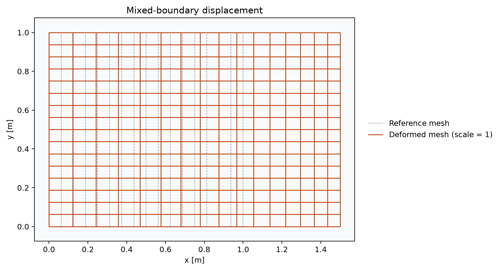

Dashed reference square and deformed mesh for a left-fixed elastic body pulled rightward by a uniform body force. — Units: mMaintained example result on a 16 × 16 Cartesian Q1 mesh, displacement scale 1. The fixed edge stays still; the right edge moves furthest.Read the plotting program

The optional --scale multiplies displacement only for display. A scale of 0.1 makes this picture less stretched; it does not reduce physical strain in the model.

Find the same equations inside reusable components

We wrote balance and traction explicitly so their meaning was visible. The standard Eqiora.Solid.LinearElasticity package supplies those same pieces:

Part of our derivation	Reusable component
$-\nabla\cdot\boldsymbol\sigma-\nabla q=0$	`IsotropicBalanceWithPotential2d`
Displacement trace and outward elastic traction	`IsotropicMechanicalInterface2d`
Zero displacement on one edge	`FixedDisplacement2d`
Zero traction on one edge	`ZeroTraction2d`

Open the component definitions. The balance contains the same symmetric displacement gradient and isotropic trace term. The interface uses that same stress on each exterior boundary. The fixed and free components supply boundary laws and connect to the interface.

The component version of this exact square is available as the composed square model. Its package binding imports Eqiora.Solid.LinearElasticity.linear_elasticity as solid; the body load remains local to the model. Read the shorter continuum component example for a complete composition walkthrough.

The convenience is now understandable: components let us reuse a material and boundary law whose equations we have already derived. Geometry, load and numerical choices remain separate decisions. Using the same $\mu$ and $\lambda$ for interior stress and boundary traction is essential; otherwise they would describe different materials at the same boundary.

Predict a change before rerunning

In the Python program, change the mu binding from 3 to 6, leaving lambda at zero. Would displacement halve? Here it will stay the same: our load definition also contains mu, so both stiffness and body load double. Reaction and stored energy double. This is different from increasing stiffness under a fixed load in the bar experiment.

Alternatively, keep geometry and coefficients fixed and change length_scale from 1 to 100. The load, displacement and reaction become one hundredth as large; stored energy becomes one ten-thousandth as large. The tip displacement is then $0.005\,\mathrm{m}$ and maximum axial strain is $0.01$ . The name length_scale belongs to the load expression; changing it does not resize the rectangle.

Exercises

Derive the reaction moment about the lower-left corner. Explain how it balances the moment of the distributed horizontal load.
Change only length_scale as above and compare the reaction vectors with your prediction. Explain why displacement and energy scale differently.
Predict what goes wrong with the one-dimensional analytic solution when lambda is made positive. Check the traction on the upper boundary first.
In the component definitions, locate the repeated stress coefficients. Explain why changing only the interface’s coefficient would be a modeling inconsistency rather than a new boundary condition.
Change only the plot scale. Name two quantities that must stay unchanged.

Reading

David Roylance, The Equilibrium Equations, MIT, September 26, 2000, especially Cauchy traction and force balance: module and PDF.
Klaus-Jürgen Bathe, Finite Element Procedures for Solids and Structures, MIT OpenCourseWare, Spring 2010, linear-analysis lecture 3, for displacement interpolation and work balance.

Previous: Virtual work · Path · Next: Reading displacement, reactions and error