Transient cylinder-flow startup

Unverified product example · Python and Colab

Gallery

This walkthrough executes ten accepted startup steps through the ordinary installed-Python lifecycle. It is deliberately not presented as a developed vortex street or a validated cylinder benchmark.

Stage 1 🧭One Geometry owner

Python authors the exact $2.2\,\mathrm{m}\times0.41\,\mathrm{m}$ channel and subtracts one exact circle. The resulting Geometry owns the fluid, inlet, outlet, walls, and cylinder selections used by meshing, compilation, and the Result observables.

python

graph = eqiora.geometry.GeometryGraph()
rectangle = graph.rectangle(x_bounds=(0.0, 2.2), y_bounds=(0.0, 0.41))
circle = graph.circle(center=(0.2, 0.2), radius=0.05)
fluid = graph.subtract(rectangle, circle)
geometry = graph.build(fluid, named_topology={...})

View the complete plain-Python workflow

Stage 2 🧩Eqiora model definition

The equations-only .eqi source owns transient incompressible Navier–Stokes meaning and abstract support names. It does not carry a second concrete shape. With velocity $\boldsymbol{u}$, density $\rho$, stress $\boldsymbol{\sigma}$, and force potential $\phi$, the momentum and incompressibility relations are

$$\rho\,\partial_t\boldsymbol{u} + \rho\,\nabla\!\cdot(\boldsymbol{u}\otimes\boldsymbol{u}) - \nabla\!\cdot\boldsymbol{\sigma} - \nabla\phi = 0, \qquad \nabla\!\cdot\boldsymbol{u}=0.$$

Open the Eqiora source

Stage 3 🔷Planning, then mesh generation

The typed Gmsh request makes the global characteristic-size target explicit. resolve only plans; generate executes Gmsh and publishes the accepted common Mesh with correspondence and production lineage.

python

request = eqiora.meshing.GmshMesher(
    maximum_boundary_error=1e-4,
    maximum_target_size=0.025,
    minimum_mean_ratio=1e-5,
    maximum_boundary_facets=50,
)
mesh_plan = eqiora.meshing.resolve(geometry, request)
mesh = eqiora.meshing.generate(mesh_plan)

A meshing choice, not convergence

0.025 m is a Gmsh characteristic target. It is not a guarantee on every realized edge and does not establish mesh or PDE convergence.

Stage 4 ▶Typed Plan, State, and Run

A steady MINI/P1 Result supplies a compatible nonzero initial State. The root resolver then combines the transient Model with typed spatial, Backward-Euler, Newton, linear, and scaling policies. One common call publishes all ten accepted startup outputs at $\Delta t=0.01\,\mathrm{s}$.

python

plan = eqiora.resolve(
    model,
    mesh=mesh,
    spatial=eqiora.fem.MiniP1(),
    temporal=eqiora.time.BackwardEuler(0.01),
    solve=eqiora.solve.Newton(linear=linear),
    scaling=eqiora.fluid.IncompressibleScaling(...),
)
result = eqiora.run(
    plan,
    state=state,
    steps=10,
    output_steps=tuple(range(1, 11)),
)

Open in Colab

The Colab entry is published beginning with the 0.1.0a4 documentation build. It opens this exact GitHub notebook in the user’s ephemeral runtime and does not depend on maintainer-owned Drive state.

Stage 5 📐Typed Result observables

The final accepted State derives cell-average vorticity, the signed intrinsic-2D cylinder action pair, and two continuous-P1 pressure samples. Each value remains bound to its exact State, Field, Mesh, selection or physical point, unit, and digest. The page reports no benchmark normalization or target value.

python

accepted = result.trajectory.state(10)
vorticity = accepted.curl(plan.capability.velocity)
cylinder_force = accepted.boundary_force(geometry.selection("cylinder"))
front_pressure = accepted.sample(plan.capability.pressure, at=(0.15, 0.2))
rear_pressure = accepted.sample(plan.capability.pressure, at=(0.25, 0.2))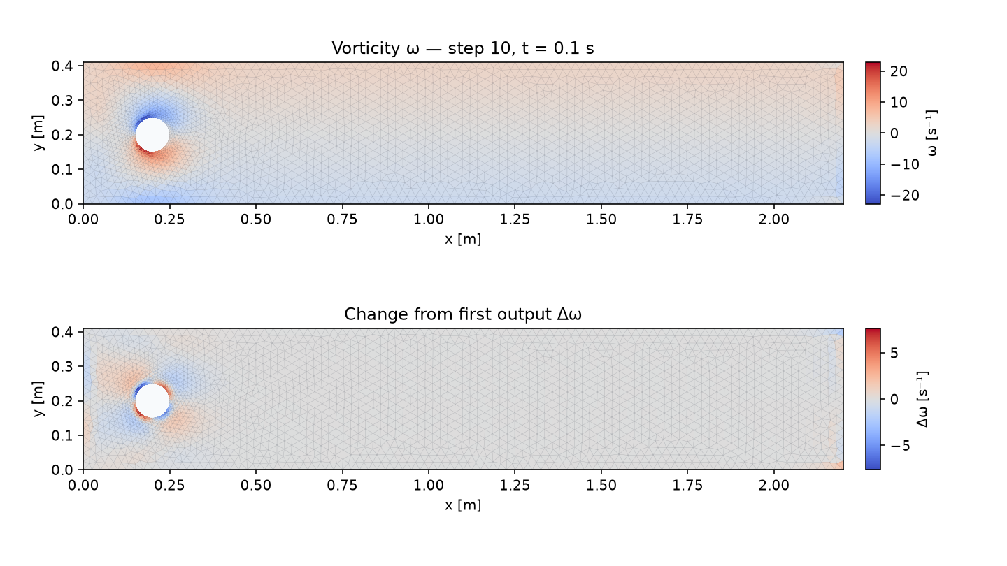

Presentation, not evidence.Units: s⁻¹Final absolute field and change from the first output at t = 0.1 s. Presentation only; the visible fields are not a benchmark or validation result.View the caller-owned media producer

Stage 6 🎞️Accessible media and product boundary

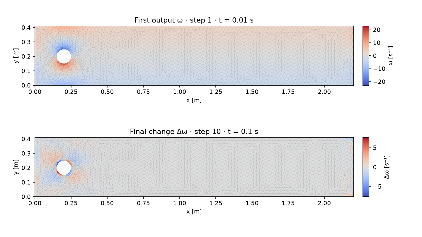
Ten actual accepted outputs, played at two frames per second so the subtle startup change remains legible. Motion is disabled when the browser requests reduced motion; the first/final still is shown instead. Presentation only, not evidence.

The right-hand panel shows Δω relative to the first output at 0.01 seconds, using one fixed symmetric scale across the sequence. By 0.1 seconds, the near-cylinder layers have intensified and extended slightly downstream. The sequence stays largely symmetric and attached. It does not show, and must not be read as, periodic shedding or a developed vortex street.

Explicitly unverified product boundary

Supported

• One installed-Python channel-minus-circle composition reaches a ten-output transient Result through exact Geometry, typed meshing and numerical policies, root resolution, State, and Run.
• Plain Python and Colab use the same public computational call order and final accepted State.
• Caller-owned poster, video, reduced-motion still, and text describe vorticity from one coherent product lineage.
• Cylinder force and pressure probes are typed Result observables; no displayed number is promoted to evidence.

Not claimed

• This startup presentation is not DFG benchmark acceptance and establishes no developed wake, shedding frequency, force, pressure, balance, or separation value.
• It makes no mesh/time convergence, performance, production-scale, 3D, turbulent, or advanced-meshing claim.
• The animation supports inspection, not scientific inference from pixels.

Read the human capability boundary

Understand and reproduce the workflow

Connect evolving state to the ODE lesson and spatial flux to conservation laws. The Python execution guide explains run control, diagnostics and array ownership. Use the Python and Colab reproductions above for this exact transient model.